This is my capstone project for the Google Data Analytics Professional Certificate. In this case study, I analyze a public dataset from Kaggle to demonstrate the technical and analytical skills acquired throughout the program. Following the core data analysis framework: Ask, Prepare, Process, Analyze, Share, and Act, I will explore user behaviors to help answer vital business questions for Bellabeat.
Founded in 2014 by Urška Sršen and Sandro Mur, Bellabeat is a high-tech wellness company that empowers women with health-focused smart technology. By tracking physical activity, sleep quality, stress levels, and reproductive health, Bellabeat provides women with personalized insights to make informed health decisions.
✓ Bellabeat App: The core digital hub tracking activity, sleep, stress, hydration, and reproductive cycles.
✓ Leaf: Bellabeat’s flagship wearable wellness tracker, designed to be worn as a necklace, clip, or bracelet.
✓ Time: A hybrid wellness watch that combines timeless aesthetic design with smart tracking technology.
✓ Spring: A smart water bottle that monitors daily hydration against user activity levels.
Project Focus: In this case study, I analyze smart device usage data from a non-Bellabeat tracker (Fitbit) to discover consumer habits and deliver data-driven marketing recommendations for the Leaf.
Analyze non-Bella beat smart device usage data to understand consumer behavior and provide strategic recommendations for the Bellabeat marketing team.
Key Stakeholders:
✓ Urška Sršen: Co-founder and Chief Creative Officer of Bellabeat.
✓ Sandro Mur: Mathematician and Co-founder of Bellabeat.
✓ Marketing Analytics Team: The dedicated team responsible for collecting, analyzing, and reporting data to guide marketing strategy.
About the Data
This dataset is titled FitBit Fitness Tracking Data and can be found on Kaggle. It is generated by respondents to a survey via Amazon Mechanical Turk over a thirty day span of time, from April 12th, 2016 to May 12th, 2016. The dataset contains the person tracking fitness data of 30 consenting users. Data includes daily steps, daily calories, a sleep log, a weight log, and more. I downloaded the data to be cleaned, analyzed, and visualized on Rstudio.
Credibility of the data
I used the ROCCC method to determine the credibility of the data:
Reliability: I would not consider this data to be reliable. The sample size is only 30, which is at the very bottom of what is considered to be a valid sample size and margin of error. This could potentially limit the amount of analysis that can be done to the data.
Originality: The dataset was originally collected by an Amazon Mechanical Turk, so it is not original.
Comprehensiveness: The dataset is not nearly as comprehensive as it could have been. There is no data on the age, gender, location, etc. This means that there is a possibility that the data could be biased. The users were not asked to wear their FitBits at all times throughout the time frame, so there is data missing within the dataset.
Current: The dataset is from 2016, so it is not current and may not fully represent what fitness tracker data may look like now.
Cited: This data is cited but doesn’t necessarily determine the credibility of the source.There are definitely limitations to this dataset. With that, this data can help provide clues and suggestions, but no concrete answers for the Bellabeat analytics team.
Credibility of the data
First, I installed and loaded the packages necessary to clean and plot the data.
install.packages("tidyverse", repos = "http://cran.us.r-project.org")
##
## The downloaded binary packages are in
## /var/folders/3w/3g5p_cbx277bdmlvy9y8yy440000gn/T//RtmptoIuN3/downloaded_packages
install.packages("dplyr", repos = "http://cran.us.r-project.org")
##
## The downloaded binary packages are in
## /var/folders/3w/3g5p_cbx277bdmlvy9y8yy440000gn/T//RtmptoIuN3/downloaded_packages
install.packages("ggplot2", repos = "http://cran.us.r-project.org")
##
## The downloaded binary packages are in
## /var/folders/3w/3g5p_cbx277bdmlvy9y8yy440000gn/T//RtmptoIuN3/downloaded_packages
install.packages("skimr", repos = "http://cran.us.r-project.org")
##
## The downloaded binary packages are in
## /var/folders/3w/3g5p_cbx277bdmlvy9y8yy440000gn/T//RtmptoIuN3/downloaded_packages
install.packages("janitor", repos = "http://cran.us.r-project.org")
##
## The downloaded binary packages are in
## /var/folders/3w/3g5p_cbx277bdmlvy9y8yy440000gn/T//RtmptoIuN3/downloaded_packages
library(tidyverse)
## ── Attaching packages ──────────────────── tidyverse 1.3.1 ──
## ✓ ggplot2 3.3.5 ✓ purrr 0.3.4
## ✓ tibble 3.1.6 ✓ dplyr 1.0.8
## ✓ tidyr 1.2.0 ✓ stringr 1.4.0
## ✓ readr 2.1.2 ✓ forcats 0.5.1
## ── Conflicts ──────────────────────────────── tidyverse_conflicts() ──
## x dplyr::filter() masks stats::filter()
## x dplyr::lag() masks stats::lag()
library(dplyr)
library(ggplot2)
library(skimr)
library(janitor)
##
## Attaching package: 'janitor'
## The following objects are masked from 'package:stats':
##
## chisq.test, fisher.test
Let’s load and name the data that we will work with. The tables I decided to work with are dailyActivity_merged.csv, weightLogInfo_merged.csv, and sleepDay_merged.csv.
setwd("~/Downloads/Fitabase Data 4.12.16-5.12.16")
daily_activity <- read.csv("dailyActivity_merged.csv")
weight_log <- read.csv("weightLogInfo_merged.csv")
sleep_log <- read.csv("sleepDay_merged.csv")
Now that we’ve got our data loaded, let’s take a closer look at the column names the data sets include.
Process
colnames(daily_activity)
## [1] "Id" "ActivityDate"
## [3] "TotalSteps" "TotalDistance"
## [5] "TrackerDistance" "LoggedActivitiesDistance"
## [7] "VeryActiveDistance" "ModeratelyActiveDistance"
## [9] "LightActiveDistance" "SedentaryActiveDistance"
## [11] "VeryActiveMinutes" "FairlyActiveMinutes"
## [13] "LightlyActiveMinutes" "SedentaryMinutes"
## [15] "Calories"
colnames(weight_log)
## [1] "Id" "Date" "WeightKg" "WeightPounds"
## [5] "Fat" "BMI" "IsManualReport" "LogId"
colnames(sleep_log)
## [1] "Id" "SleepDay" "TotalSleepRecords"
## [4] "TotalMinutesAsleep" "TotalTimeInBed"
The head function gives us the ability to see the first few rows in each dataset.
head(daily_activity)
## Id ActivityDate TotalSteps TotalDistance TrackerDistance
## 1 1503960366 4/12/2016 13162 8.50 8.50
## 2 1503960366 4/13/2016 10735 6.97 6.97
## 3 1503960366 4/14/2016 10460 6.74 6.74
## 4 1503960366 4/15/2016 9762 6.28 6.28
## 5 1503960366 4/16/2016 12669 8.16 8.16
## 6 1503960366 4/17/2016 9705 6.48 6.48
## LoggedActivitiesDistance VeryActiveDistance ModeratelyActiveDistance
## 1 0 1.88 0.55
## 2 0 1.57 0.69
## 3 0 2.44 0.40
## 4 0 2.14 1.26
## 5 0 2.71 0.41
## 6 0 3.19 0.78
## LightActiveDistance SedentaryActiveDistance VeryActiveMinutes
## 1 6.06 0 25
## 2 4.71 0 21
## 3 3.91 0 30
## 4 2.83 0 29
## 5 5.04 0 36
## 6 2.51 0 38
## FairlyActiveMinutes LightlyActiveMinutes SedentaryMinutes Calories
## 1 13 328 728 1985
## 2 19 217 776 1797
## 3 11 181 1218 1776
## 4 34 209 726 1745
## 5 10 221 773 1863
## 6 20 164 539 1728
head(weight_log)
## Id Date WeightKg WeightPounds Fat BMI
## 1 1503960366 5/2/2016 11:59:59 PM 52.6 115.9631 22 22.65
## 2 1503960366 5/3/2016 11:59:59 PM 52.6 115.9631 NA 22.65
## 3 1927972279 4/13/2016 1:08:52 AM 133.5 294.3171 NA 47.54
## 4 2873212765 4/21/2016 11:59:59 PM 56.7 125.0021 NA 21.45
## 5 2873212765 5/12/2016 11:59:59 PM 57.3 126.3249 NA 21.69
## 6 4319703577 4/17/2016 11:59:59 PM 72.4 159.6147 25 27.45
## IsManualReport LogId
## 1 True 1.462234e+12
## 2 True 1.462320e+12
## 3 False 1.460510e+12
## 4 True 1.461283e+12
## 5 True 1.463098e+12
## 6 True 1.460938e+12
head(sleep_log)
## Id SleepDay TotalSleepRecords TotalMinutesAsleep
## 1 1503960366 4/12/2016 12:00:00 AM 1 327
## 2 1503960366 4/13/2016 12:00:00 AM 2 384
## 3 1503960366 4/15/2016 12:00:00 AM 1 412
## 4 1503960366 4/16/2016 12:00:00 AM 2 340
## 5 1503960366 4/17/2016 12:00:00 AM 1 700
## 6 1503960366 4/19/2016 12:00:00 AM 1 304
## TotalTimeInBed
## 1 346
## 2 407
## 3 442
## 4 367
## 5 712
## 6 320
By using n_distinct function, I can get a count of how many distinct values are in the data sets’ ID columns.
n_distinct(daily_activity$Id)
## [1] 33
n_distinct(weight_log$Id)
## [1] 8
n_distinct(sleep_log$Id)
## [1] 24
From the number of distinct ID’s entered in the three data sets, there were much less people who manually entered their data.Now, to check for duplicates, let’s get a count on the total number of rows in the data sets.
nrow(daily_activity)
## [1] 940
nrow(weight_log)
## [1] 67
nrow(sleep_log)
## [1] 413
To ensure the data is not skewed, let’s check to see if there are any duplicates in our data frames.
nrow(daily_activity[duplicated(daily_activity),])
## [1] 0
nrow(weight_log[duplicated(weight_log),])
## [1] 0
nrow(sleep_log[duplicated(sleep_log),])
## [1] 3
There are three duplicates in our sleep log. I am going to create a new sleep log data frame that only includes unique entries.
sleep_log_new <- unique(sleep_log)
Just to be sure, let’s check our new data frame to look for any duplicates.
nrow(sleep_log_new[duplicated(sleep_log_new),])
## [1] 0
There should now be 410 observations in our sleep log
nrow(sleep_log_new)
## [1] 410
Finally, I would like to check the total number of zero entries their are in the Calories column, this helps me see how many days that users weren’t wearing their device and logging in any data.
Analyze
Now that the data is loaded and clean, let’s look at the datas’ summary statistics.
daily_activity %>%
select (TotalSteps,
TotalDistance,
VeryActiveMinutes,
FairlyActiveMinutes,
LightlyActiveMinutes,
SedentaryMinutes,
Calories) %>%
summary ()
## TotalSteps TotalDistance VeryActiveMinutes FairlyActiveMinutes
## Min. : 0 Min. : 0.000 Min. : 0.00 Min. : 0.00
## 1st Qu.: 3790 1st Qu.: 2.620 1st Qu.: 0.00 1st Qu.: 0.00
## Median : 7406 Median : 5.245 Median : 4.00 Median : 6.00
## Mean : 7638 Mean : 5.490 Mean : 21.16 Mean : 13.56
## 3rd Qu.:10727 3rd Qu.: 7.713 3rd Qu.: 32.00 3rd Qu.: 19.00
## Max. :36019 Max. :28.030 Max. :210.00 Max. :143.00
## LightlyActiveMinutes SedentaryMinutes Calories
## Min. : 0. 0 Min. : 0. 0 Min. : 0
## 1st Qu.:127.0 1st Qu.: 729.8 1st Qu.:1828
## Median :199.0 Median :1057.5 Median :2134
## Mean :192.8 Mean : 991.2 Mean :2304
## 3rd Qu.:264.0 3rd Qu.:1229.5 3rd Qu.:2793
## Max. :518.0 Max. :1440.0 Max. :4900
sleep_log_new %>%
select (TotalSleepRecords,
TotalMinutesAsleep,
TotalTimeInBed) %>%
summary ()
## TotalSleepRecords TotalMinutesAsleep TotalTimeInBed
## Min. :1.00 Min. : 58.0 Min. : 61.0
## 1st Qu.:1.00 1st Qu.:361.0 1st Qu.:403.8
## Median :1.00 Median :432.5 Median :463.0
## Mean :1.12 Mean :419.2 Mean :458.5
## 3rd Qu.:1.00 3rd Qu.:490.0 3rd Qu.:526.0
## Max. :3.00 Max. :796.0 Max. :961.0
weight_log %>%
select (WeightPounds,
BMI) %>%
summary ()
## WeightPounds BMI
## Min. :116.0 Min. :21.45
## 1st Qu.:135.4 1st Qu.:23.96
## Median :137.8 Median :24.39
## Mean :158.8 Mean :25.19
## 3rd Qu.:187.5 3rd Qu.:25.56
## Max. :294.3 Max. :47.54
Share: Visualizations
Let’s plot some of our findings!First, I want to analyze the relationship between total steps and calories.
ggplot(data = daily_activity) +
geom_point(mapping=aes(x=TotalSteps, y=Calories, color= VeryActiveMinutes)) +
labs(title = "Relationship Between Total Steps and Calories", x = "Total Steps", y = "Calories Burned")
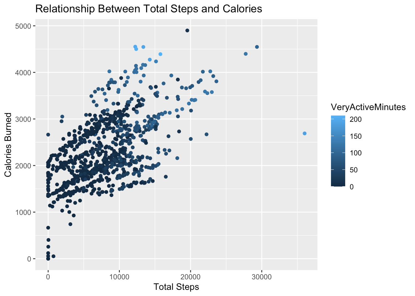
correlation between steps taken and calories. The more steps taken, the more calories are burned. Adding the Very Active Minutes as the scale shows the more active minutes a user has, the more calories they burn.
Next, let’s examine the relationship between Total Steps and Sedentary Minutes
ggplot(data = daily_activity) +
geom_point(mapping = aes(x = TotalSteps, y = SedentaryMinutes,color = Calories)) +
geom_smooth(mapping=aes(x=TotalSteps, y=SedentaryMinutes)) +
labs(title = "Relationship Between Total Steps and Sedentary Minutes", x = "Total Steps", y = "Sedentary Minutes")
## `geom_smooth()` using method = 'loess' and formula 'y ~ x'
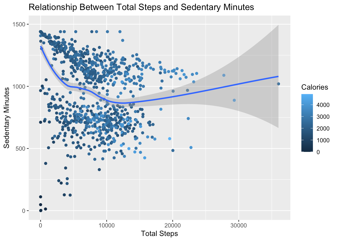
steps taken, the more sedentary minutes the user has. Overall, users were not spending a lot of time being active.
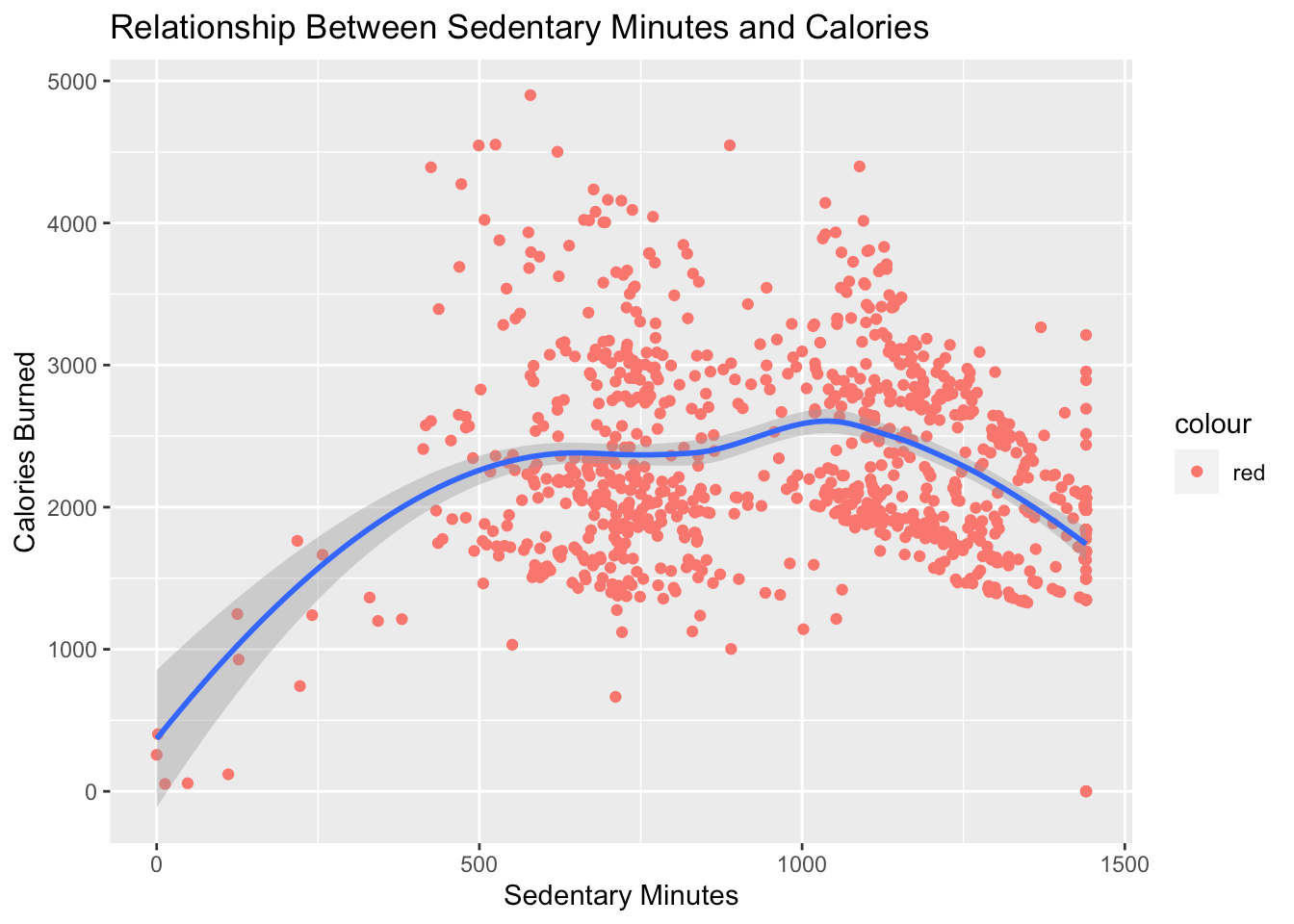
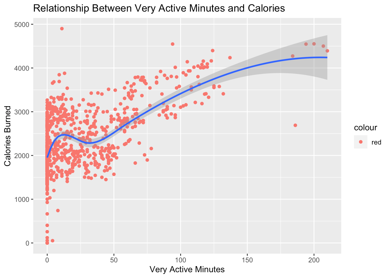
Next, let’s compare the relationships between Sedentary Minutes and Calories and Very Active Minutes and Calories.
ggplot(data = daily_activity) +
geom_point(mapping = aes(x= SedentaryMinutes, y = Calories, color = "red")) +
geom_smooth(mapping=aes(x=SedentaryMinutes, y=Calories)) +
labs(title = "Relationship Between Sedentary Minutes and Calories", x = "Sedentary Minutes", y = "Calories Burned")
## `geom_smooth()` using method = 'loess' and formula 'y ~ x'
ggplot(data = daily_activity) +
geom_point(mapping = aes(x= VeryActiveMinutes, y = Calories, color = "red")) +
geom_smooth(mapping=aes(x=VeryActiveMinutes, y=Calories)) +
labs(title = "Relationship Between Very Active Minutes and Calories", x = "Very Active Minutes", y = "Calories Burned")
## `geom_smooth()` using method = 'loess' and formula 'y ~ x'
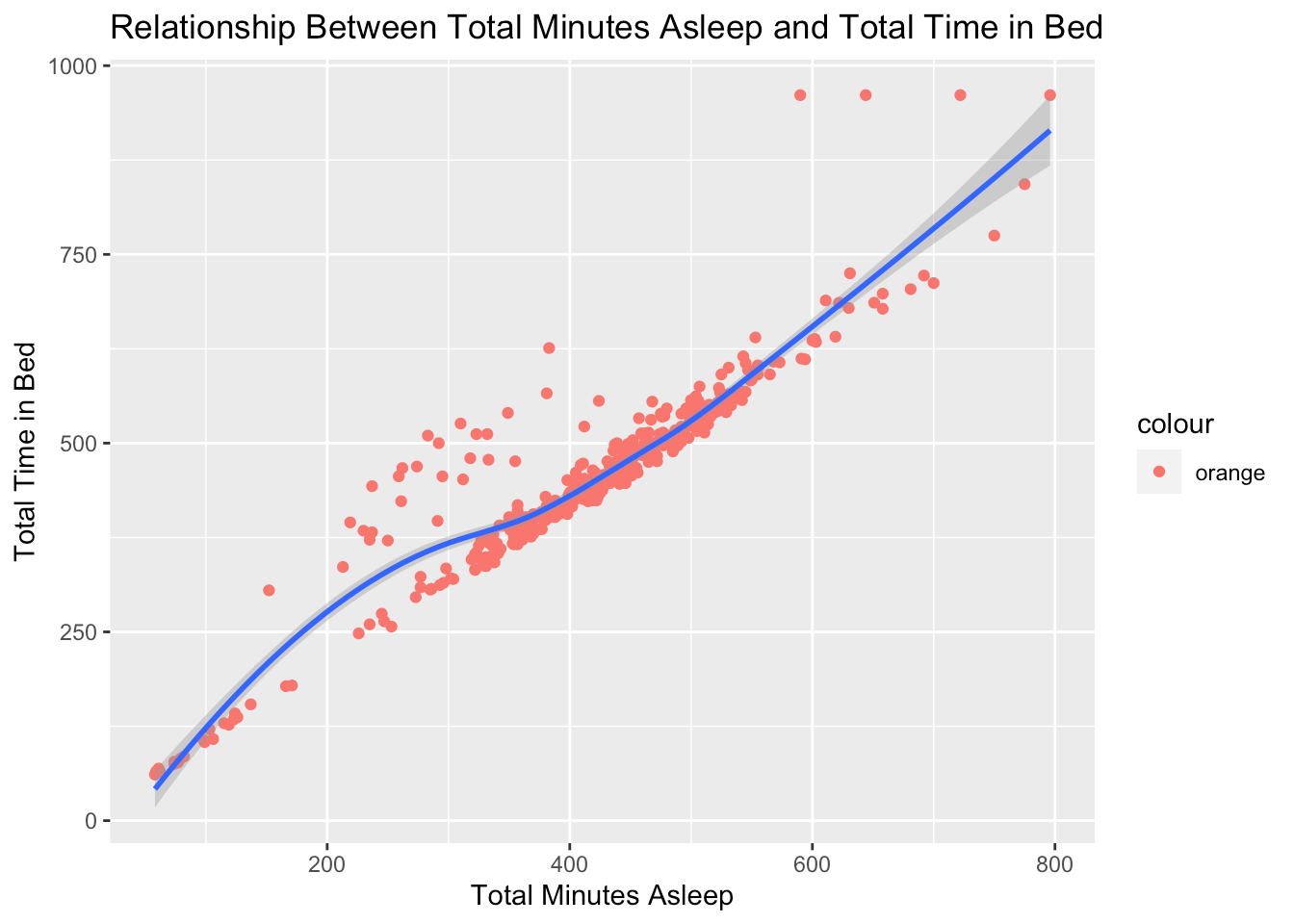
between minutes slept and time in bed
ggplot(data = sleep_log_new) +
geom_point(mapping = aes(x = TotalMinutesAsleep, y = TotalTimeInBed, color = "orange")) +
geom_smooth(mapping = aes(x = TotalMinutesAsleep, y = TotalTimeInBed)) +
labs (title = "Relationship Between Total Minutes Asleep and Total Time in Bed", x = "Total Minutes Asleep", y = "Total Time in Bed")
## `geom_smooth()` using method = 'loess' and formula 'y ~ x'